Doing Science Using Open Data – Part 7: Modelling Populations 2

 

In the third part in this series I looked at the UK mid-2011 Census and obtained the data below which represents the summed male and female figures for the UK population from ages 16 through to 44.

680,979
706,234
711,491
741,667
765,895
757,901
757,295
771,297
756,449
768,415
774,921
759,889
768,860
770,810
778,986
782,510
751,251
700,825
690,775
702,024
716,419
729,013
761,347
794,300
820,805
800,550
821,037
819,650
832,297

Data for this group and the 45-65 year age group are graphed in Figure 1.

 

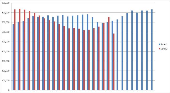
Figure 1: Summation of male and female figures for each age from mid-2011 Census. Red bars represent the age group 45-65 and the blue bars represent the age group 16-44

The next stage is to try and model this data. Looking at the blue bars in the graph above, it looks as though there is some periodicity in the data. This isn’t a great approximation but the bimodal distribution can be seen below where the peaks and troughs of the data are shown by the horizontal black lines.

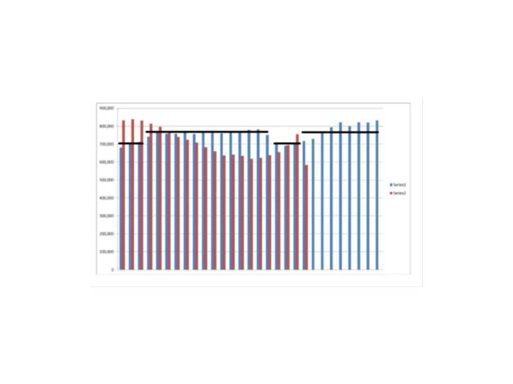
Figure 2

In this approximation of the data there are 3 troughs for every 14 peaks in the data (counting the bars). Initially I thought to represent this as a rectangular pulse and to use a Fourier transform but this was slightly tricky (for me). As there is periodicity in the data I thought it might be possible to use sine and cosine functions. The graph below shows a light wave divided into its electromagnetic components along different axes. Focusing on one axis its possible to see that the wave can be described by an amplitude (i.e the height that the wave reaches) and a wavelength (the distance along the x-axis during one cycle – denoted here by lambda).

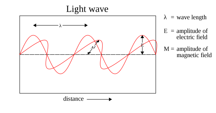
Figure 3 – A Lightwave

Returning to the data above one approximation that looked promising was y = cos (theta) + sin(theta/2) as this produces wide peaks and narrow troughs. Then it should be a simple matter of increasing the amplitude by introducing a coefficient and adding a constant. However the problem is that the ratio of peak width to trough width needs to be 14/3 or approximately 4.6. The sine/cosine graph has a ratio which is much less than this which means it doesn’t fit the data well.

For the moment then the graph can be described by a discontinuous function

1. For X = 16-18, Y = 700,000

2. For X = 19-32, Y = 770,000

3. For X = 33-35, Y = 700,000

4. For X = 36-45, Y = 770,000

This is a simple rectangle function. For the age group 36-45, the Y value could be a little higher but I am approximating a simple fit to the data. As soon as i’ve figured out a function which incorporates periodicity i’ll replace this rectangle function (or if any of the readers work it out – please let me know). For the time being however the above graphs describe the UK mid-2011 census data for the age group 16-45.

Appendix

Doing Science Using Open Data – Part 1

Doing Science Using Open Data – Part 2

Doing Science Using Open Data – Part 3

Doing Science Using Open Data – Part 4

Doing Science Using Open Data – Part 5

Doing Science Using Open Data – Part 6

Index: There are indices for the TAWOP site here and here Twitter: You can follow ‘The Amazing World of Psychiatry’ Twitter by clicking on this link. Podcast: You can listen to this post on Odiogo by clicking on this link (there may be a small delay between publishing of the blog article and the availability of the podcast). It is available for a limited period. TAWOP Channel: You can follow the TAWOP Channel on YouTube by clicking on this link. Responses: If you have any comments, you can leave them below or alternatively e-mail justinmarley17@yahoo.co.uk. Disclaimer: The comments made here represent the opinions of the author and do not represent the profession or any body/organisation. The comments made here are not meant as a source of medical advice and those seeking medical advice are advised to consult with their own doctor. The author is not responsible for the contents of any external sites that are linked to in this blog.